BEA County Income & Employment Summary, 2008

2008 estimates from the BEA County Income and Employment Summary HealthLandscape.

Bureau of Economic Analysis data released in April of 2010 are new estimates for 2008.

The first part of Table CA04 presents the summary statistics: Personal income, nonfarm personal income, farm income, population (estimated as of July 1 of each year by the Census Bureau), and per capita personal income, which is personal income divided by population.

The second part of Table CA04 presents the derivation of personal income. Personal income is measured as the sum of wages and salaries; supplements to wages and salaries; proprietors' income; dividends, interest, and rent; and personal current transfer receipts; less contributions for government social insurance. The personal income of a local area is defined as the income received by the residents of the local area, but the estimates of wages and salaries, supplements to wages and salaries, and contributions for government social insurance by employees are based mainly on source data that are reported not by the place of residence of the income recipients but by their place of work. Accordingly, an adjustment for residence-- which is the net inflow of the earnings of wage and salary workers who are interstate commuters-- is estimated so that place-of-residence measures of earnings and personal income can be derived. Net earnings by place of residence is calculated by subtracting contributions for government social insurance from earnings by place of work and then adding the adjustment for residence. The estimates of dividends, interest, and rent, and of personal current transfer receipts are prepared by place of residence only.

The third part of Table CA04 presents the summary estimates of total employment, wage and salary employment, and proprietors employment.

For more information, see BEA Regional Economic Accounts.

Figure 1. Per Capita Personal Income (Dollars), 2008


Figure 2. Non-Farm Personal Income, 2008

Login now to start making maps!

Show the need.

Paint a portrait.

Tell the story.

Appalachian Economic Status Data Updates

Economic Status Data are now available for fiscal years 2010 and 2011.

The Appalachian region is home to 24.8 million people and consists of 420 counties across 13 states, stretching from New York and Pennsylvania in the northeast to Mississippi and Alabama in the south. Forty-two percent of the Region's population is rural, compared with 20 percent of the national population. The Appalachian population is characterized by lower levels of college completion and lower labor force participation. Southern areas of Appalachia attract better educated and higher skilled people.

In recent years, the region's economy has become more diversified, rather than relying on mining, forestry, agriculture, chemical industries, and heavy industry. In 1965, one in three Appalachians lived in poverty. In 2000, the Region's poverty rate was 13.6 percent.

The Appalachian Regional Commission (ARC) categorizes each county in the region into one of five economic levels: distressed, at-risk, transitional, competitive, and attainment. The system involves the creation of a national index of county economic status through a comparison of each county's averages for three economic indicators--three-year average unemployment rate, per capita market income, and poverty rate--with national averages. In 1965, 223 Appalachian counties were considered economically distressed. In fiscal year 2011 that number is 82. For more informatoin on how the ARC defines the economic categories, visit their website.

Figure 1. Applachian Economic Status, FY2011




The ARC uses US Bureau of Labor Statistics unemployment rates as a part of its economic classification system. The three-year average unemployment rate is a measure of long-term structural unemployment that allows for the comparison of counties across state borders. The unemployment rate is calculated by dividing the three-year sum of persons unemployed by the three-year sum of the civilian labor force.

Figure 2. Applachian Three-year Unemployment Rate 2006-2008



These data, and others for Appalachia, are now available in HealthLandscape for use in your maps. You can find these data by going to Community HealthView → United States → Appalachian Counties Economic Status.

Login now to start making maps!

Show the need.

Paint a portrait.

Tell the story.

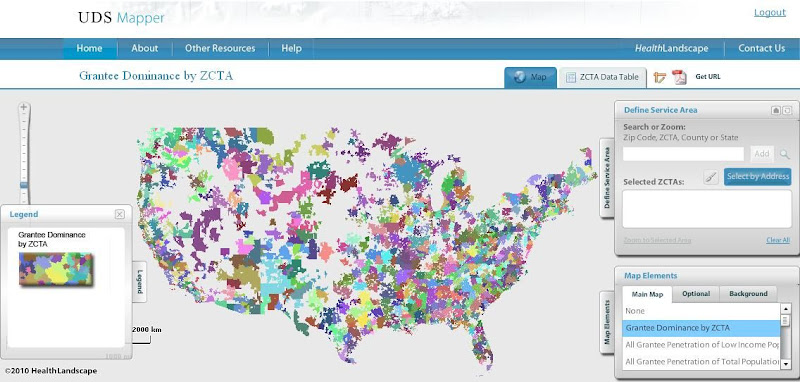
HealthLandscape Presents the UDS Mapper

HealthLandscape is pleased to present an additional tool within its online platform: the UDS Mapper

In a period of landmark health system reform and safety net expansion, it is essential that accessible tools and data are available to assist in evaluating the geographic extent of federally (Section 330)-supported health centers. As such, HRSA, John Snow, Inc. and the Robert Graham Center collaborated to develop this mapping and decision-support tool which is driven primarily from data within the Uniform Data System (UDS), previously not publicly accessible at the local level.






Register for access to the UDS Mapper at www.UDSMapper.org. Webinars to demonstrate the functionality of this tool will be offered weekly through August and September. Links to register for these webinars and other help tools can be found at http://www.udsmapper.org/webinars.cfm.

Commute to Work and Class of Worker

Two indicators from the American Community Survey (ACS) 2006-2008 Estimates are now available in HealthLandscape.

The data on means of transportation to work refer to the principal mode of travel or type of conveyance that the worker usually used to get from home to work during the reference week. People who used different means of transportation on different days of the week were asked to specify the one they used most often, that is, the greatest number of days. People who used more than one means of transportation to get to work each day were asked to report the one used for the longest distance during the work trip. The category "Car, Truck or Van" includes workers using a car (including company cars, but excluding taxicabs), a truck of one-ton capacity or less, or a van. The category "Public Transportation" includes workers who used a bus or trolley bus, streetcar or trolley car, subway or elevated, railroad, or ferryboat, even if each mode is not shown separately in the tabulation. The category "Other Means" includes workers who used a mode of travel that is not identified separately within the data distribution.

Figure 1. Mean Travel Time to Work


Figure 2. Percent Using Public Transportation


The ACS Estimates on class of worker categorizes people according to the type of ownership of the employing organization. For employed people, the data refer to the person’s job during the previous week. For those who worked two or more jobs, the data refer to the job where the person worked the greatest number of hours. For unemployed people, the data refer to their last job. Respondents provided the data for the tabulations by writing on the questionnaires descriptions of their kind of business or industry and the kind of work or occupation they are doing.

Figure 3. Percent Private Wage and Salary Workers


For more information on these indicators, see American Community Survey and 2008 Subject Definitions.

Login now to start making maps!

Show the need.

Paint a portrait.

Tell the story.

Crime by State, 2008

New data available in HealthLandscape!

The FBI collects these data through the Uniform Crime Reporting (UCR) Program.

Data provides the rate of selected offenses per 100,000 inhabitants for each state.

Any comparisons of crime among different locales should take into consideration relevant factors in addition to the area's crime statistics. Variables Affecting Crime provides more details concerning the proper use of UCR statistics.

For more information, see 2008 Crime in the United States, Data Declaration.


Figure 1. Violent Crime Per 100,000 Inhabitants, 2008



Figure 2. Property Crime Per 100,000 Inhabitants, 2008

Login now to start making maps!

Show the need.

Paint a portrait.

Tell the story.

USDA Food Environment Atlas

New data available in HealthLandscape!

County-level data from the USDA Food Environment Atlas is now available in HealthLandscape. The Food Environment Atlas includes data on proximity to food stores and restaurants, food prices, nutrtion-related assistance programs, health, and community characteristics. These factors interact to influence food choices and diet quality. The Atlas was developed to centralize food- and nutrition-related information and provide a spatial overview of these statistics.

The Atlas is made up of three main categories. The Food Choices category includes information on access to healthy and affordable food. Some examples of indicators in this category include access and proximity to a grocery store, the number of fast-food restaurants, access to local foods, food assistance program participation, and availability of local foods.

Figure 1. Percent of Households with No Car and > 1 Mile from Grocery Store


Figure 2. WIC-Authorized Stores per 1000 Population


Figure 3. Number of Fast Food Restaurants



Health and Well-Being indicators contain information on the community's health and diets, including rates of diabetes and obesity, and physical activity levels.

Figure 4. Adult Obesity Rate



Community Characteristics are aspects of the community that can have an influence on the food environment, including the demographic composition, income and poverty statistics, and the number of recreation and fitness centers available to the population.

Figure 5. Percent of Students Free-Lunch Eligible

Login now to start making maps!

Show the need.

Paint a portrait.

Tell the story.